5.2.4 决策树

本节概览

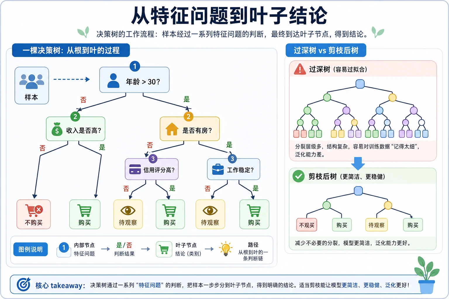
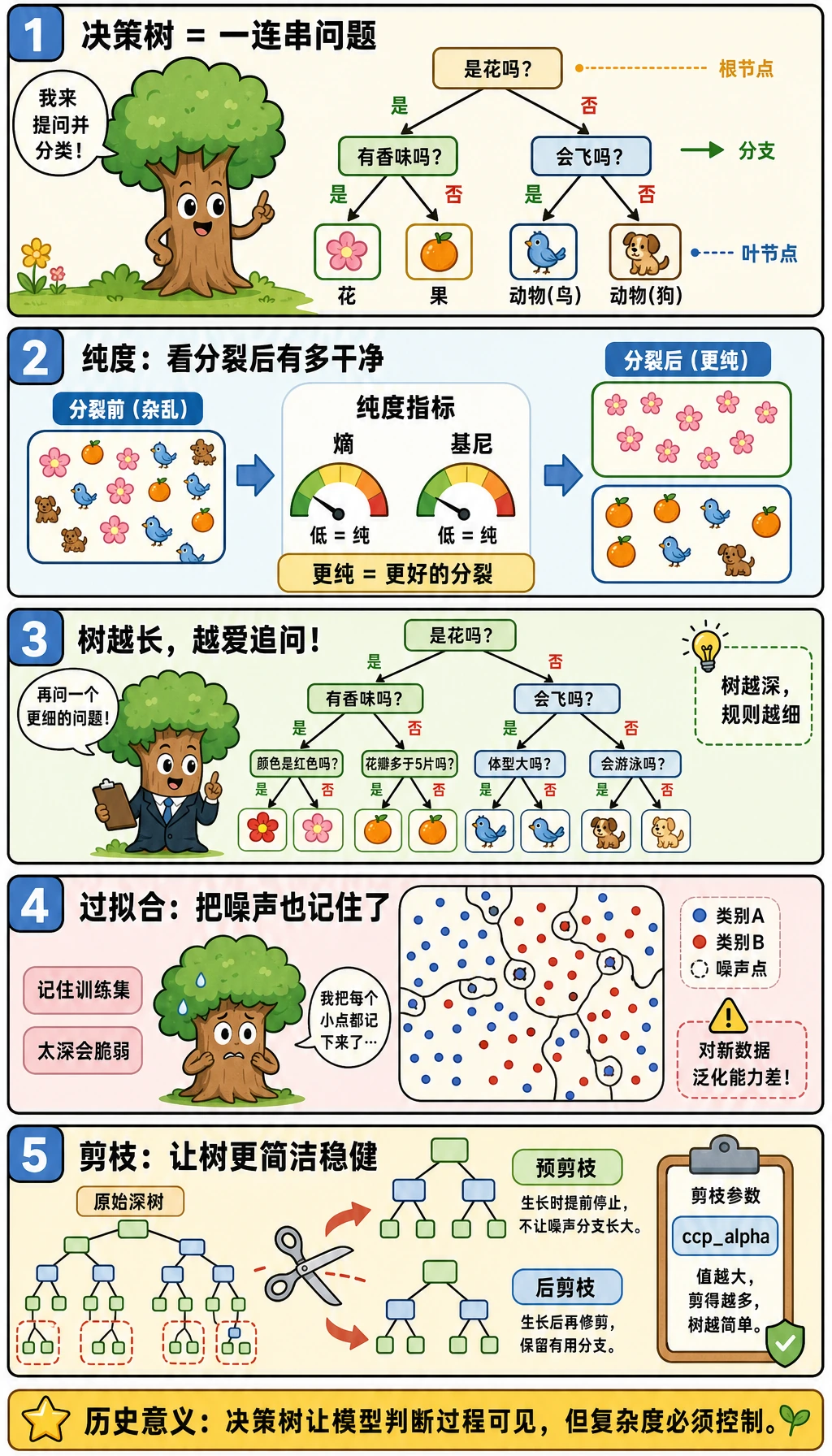
决策树是由一连串问题组成的模型。它容易读懂，因为每个预测都会沿着规则路径往下走；但如果规则过细，它也很容易过拟合。

你会做出什么

这一节会通过一个脚本演示：

• 树的深度如何影响训练集/测试集准确率；
• 如何打印可读的树规则；
• 特征重要性如何来自划分；
• ccp_alpha 后剪枝如何改变叶子数量；
• 回归树如何做出阶梯状的数值预测。

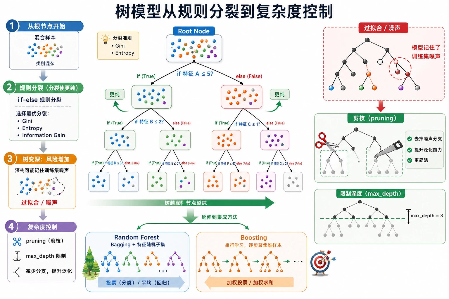
先看图。决策树不是简单的 “if-else”，而是 “if-else + 划分评分 + 复杂度控制”。

环境准备

python -m pip install -U scikit-learn

本节使用 sklearn 的 CART 风格 DecisionTreeClassifier 和 DecisionTreeRegressor。CART 是 Classification and Regression Trees，分类与回归树，意思是同一套树思想既能处理类别，也能处理数值。

运行完整实验

新建 decision_tree_lab.py：

from sklearn.datasets import load_diabetes, load_iris
from sklearn.metrics import accuracy_score, mean_absolute_error
from sklearn.model_selection import train_test_split
from sklearn.tree import DecisionTreeClassifier, DecisionTreeRegressor, export_text


iris = load_iris()
X = iris.data[:, 2:4]  # petal length and petal width, easier to read
y = iris.target
X_train, X_test, y_train, y_test = train_test_split(
    X, y, test_size=0.25, random_state=42, stratify=y
)

print("classification_depth_lab")
for depth in [1, 2, 3, None]:
    tree = DecisionTreeClassifier(max_depth=depth, min_samples_leaf=3, random_state=42)
    tree.fit(X_train, y_train)
    train_acc = accuracy_score(y_train, tree.predict(X_train))
    test_acc = accuracy_score(y_test, tree.predict(X_test))
    print(
        f"max_depth={str(depth):<4} "
        f"train={train_acc:.3f} test={test_acc:.3f} "
        f"leaves={tree.get_n_leaves()} depth={tree.get_depth()}"
    )

best_tree = DecisionTreeClassifier(max_depth=3, min_samples_leaf=3, random_state=42)
best_tree.fit(X_train, y_train)
print("tree_rules")
print(export_text(best_tree, feature_names=["petal length", "petal width"], decimals=2, max_depth=3))

print("feature_importance")
for name, value in zip(["petal length", "petal width"], best_tree.feature_importances_):
    print(f"- {name}: {value:.3f}")

print("pruning_lab")
path = DecisionTreeClassifier(random_state=42).cost_complexity_pruning_path(X_train, y_train)
for alpha in path.ccp_alphas[[0, 1, -2]]:
    pruned = DecisionTreeClassifier(random_state=42, ccp_alpha=float(alpha))
    pruned.fit(X_train, y_train)
    print(
        f"ccp_alpha={alpha:.4f} "
        f"test={accuracy_score(y_test, pruned.predict(X_test)):.3f} "
        f"leaves={pruned.get_n_leaves()}"
    )

print("regression_tree_lab")
diabetes = load_diabetes()
X_train, X_test, y_train, y_test = train_test_split(
    diabetes.data, diabetes.target, test_size=0.25, random_state=42
)
for depth in [2, 4, None]:
    reg = DecisionTreeRegressor(max_depth=depth, min_samples_leaf=10, random_state=42)
    reg.fit(X_train, y_train)
    pred = reg.predict(X_test)
    print(f"max_depth={str(depth):<4} mae={mean_absolute_error(y_test, pred):.1f} leaves={reg.get_n_leaves()}")

运行：

python decision_tree_lab.py

预期输出：

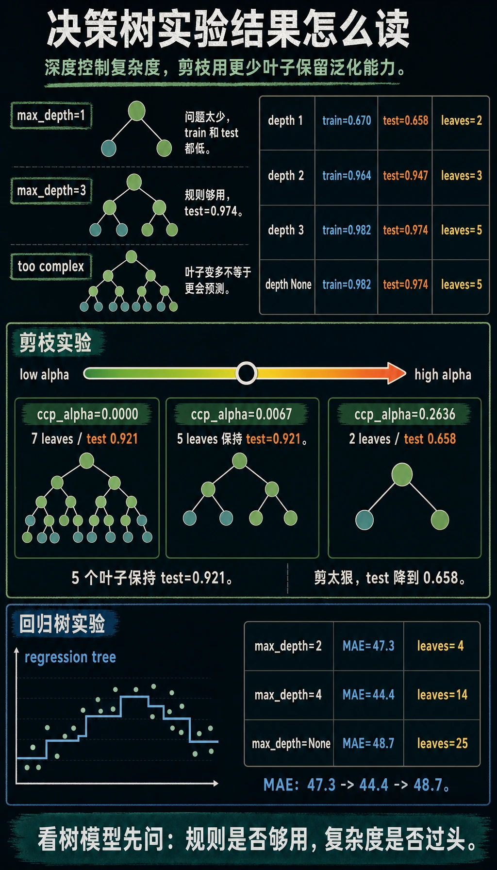
classification_depth_lab
max_depth=1    train=0.670 test=0.658 leaves=2 depth=1
max_depth=2    train=0.964 test=0.947 leaves=3 depth=2
max_depth=3    train=0.982 test=0.974 leaves=5 depth=3
max_depth=None train=0.982 test=0.974 leaves=5 depth=3
tree_rules
|--- petal length <= 2.45
|   |--- class: 0
|--- petal length >  2.45
|   |--- petal width <= 1.70
|   |   |--- petal length <= 4.95
|   |   |   |--- class: 1
|   |   |--- petal length >  4.95
|   |   |   |--- class: 2
|   |--- petal width >  1.70
|   |   |--- petal length <= 4.95
|   |   |   |--- class: 2
|   |   |--- petal length >  4.95
|   |   |   |--- class: 2

feature_importance
- petal length: 0.588
- petal width: 0.412
pruning_lab
ccp_alpha=0.0000 test=0.921 leaves=7
ccp_alpha=0.0067 test=0.921 leaves=5
ccp_alpha=0.2636 test=0.658 leaves=2
regression_tree_lab
max_depth=2    mae=47.3 leaves=4
max_depth=4    mae=44.4 leaves=14
max_depth=None mae=48.7 leaves=25

读懂输出

第一段最重要：

max_depth=1    train=0.670 test=0.658 leaves=2 depth=1
max_depth=3    train=0.982 test=0.974 leaves=5 depth=3

max_depth=1 只问一个问题，模型太简单。max_depth=3 会继续追问几轮，效果明显更好。在这个小数据集上，max_depth=None 没有继续长得更深，因为 min_samples_leaf=3 限制了过小叶子，而且数据本身比较简单。

每个节点都会寻找这样的问题：

petal length <= 2.45?

好的划分会让子节点比父节点更“干净”。干净的意思是，一个节点里的标签更少混杂。

Gini、熵与信息增益

第一次学习时，不需要立刻背所有公式。先记住它们的工作：

术语	实用含义
Gini	衡量节点里标签有多混杂；sklearn 分类树默认值
entropy	另一种混杂程度评分，和信息论有关
information gain	划分后混杂程度下降了多少
criterion	选择评分规则的参数，例如 criterion="gini" 或 criterion="entropy"

没有特殊理由时，先用 gini。很多表格项目里，调树深、叶子大小和剪枝，比把 Gini 换成 entropy 更关键。

控制复杂度

实操调参顺序：

1. 先设置 max_depth，防止树长得过深。
2. 再设置 min_samples_leaf，让每个叶子至少有足够样本。
3. 最后用 ccp_alpha 对已经长出来的树做后剪枝。

剪枝输出展示了取舍：

ccp_alpha=0.0000 test=0.921 leaves=7
ccp_alpha=0.0067 test=0.921 leaves=5
ccp_alpha=0.2636 test=0.658 leaves=2

轻微剪枝保留了测试分数，同时叶子更少。剪得太重时，树只剩两个叶子，很多有用规则也丢了。

解释性

export_text() 会打印样本会走过的规则路径。给同事解释预测原因时很有用：

|--- petal length <= 2.45
|   |--- class: 0

特征重要性也有价值，但要谨慎：

• 它表示这个已训练树中，哪些特征降低纯度最多；
• 它可能偏爱可划分点更多的特征；
• 相关特征之间会分摊或掩盖重要性；
• 它不等于因果重要性。

后面做更严谨解释时，可以把树的重要性和 permutation importance 对照。

回归树

回归树预测数值，但思想相同：把特征空间切成多个区域，然后每个叶子输出目标值平均数。

所以回归树的预测常常像阶梯，而不是光滑直线。实验里：

max_depth=4    mae=44.4 leaves=14
max_depth=None mae=48.7 leaves=25

更深的树叶子更多，但测试 MAE 反而更差。规则更多不等于泛化更好。

什么时候用单棵决策树

适合使用单棵树的场景：

• 需要一个快速、可解释的基线；
• 需要把模型规则提取给业务流程；
• 想用可视化方式解释非线性划分；
• 作为 Random Forest 或 boosting 前的垫脚石。

不建议只依赖单棵树的场景：

• 数据稍微变化，树结构就大变；
• 测试分数远低于训练分数；
• 问题需要集成模型的准确性和稳定性。

常见排查清单

现象	可能原因	修复方式
训练分数高，测试分数低	树太深	降低 max_depth，提高 min_samples_leaf，尝试剪枝
叶子很多且很小	正在记住少数特殊样本	提高 min_samples_leaf
特征重要性不可信	特征相关或高基数特征影响	用 permutation importance 复核
规则难读	树太大	训练一棵更小的解释树，或只总结关键路径
回归树预测像一格一格的台阶	叶子平均值导致阶梯输出	对比线性模型、随机森林或梯度提升

练习

1. 把 min_samples_leaf 从 3 改成 1，再改成 10。叶子数和测试准确率怎么变？
2. 把 criterion 改成 "entropy"。第一层划分还一样吗？
3. 打印 max_depth=2 的 export_text()。是不是更容易解释？
4. Iris 改成使用四个特征。特征重要性会变化吗？
5. 在回归树部分，把结果和线性回归课程里的基线对比。

过关检查

你能解释下面几点，就完成本节：

• 树通过选择让子节点更干净的划分来学习；
• 树越深，越容易记住训练集；
• max_depth、min_samples_leaf、ccp_alpha 都在控制复杂度；
• 特征重要性有用，但不等于因果关系；
• 回归树输出叶子平均值，所以预测常呈阶梯状。