5.1.6 Scikit-learn と Matplotlib 実践ワークショップ

この節の位置づけ

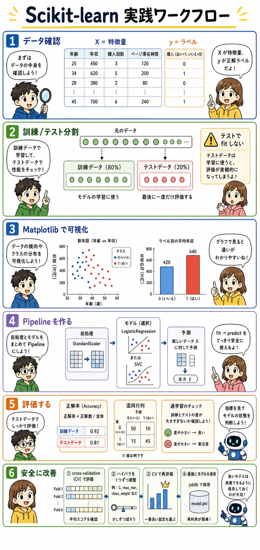
この節は手を動かすワークショップです。新しい理論を増やすことではなく、データを読む、まず図を見る、分割する、モデルを学習する、評価する、安全に改善する、保存する、という一連の流れを自分で実行できるようにします。

学習目標

• X、y、X_train、X_test、y_train、y_test が実コードで何を意味するか理解する
• Matplotlib でデータと結果を見てからスコアを信じる習慣を作る
• 前処理とモデルをまとめた sklearn Pipeline を作る
• 訓練スコアとテストスコアを比べ、過学習に気づけるようになる
• 交差検証を使い、1つずつ安全に調整する
• joblib で学習済み Pipeline を保存・再読み込みする

まず実行用セルを準備する

新しい Notebook または Python ファイルを作り、最初に次を実行します。

import numpy as np
import matplotlib.pyplot as plt

from sklearn.datasets import load_wine
from sklearn.model_selection import train_test_split, cross_val_score
from sklearn.pipeline import make_pipeline
from sklearn.preprocessing import StandardScaler
from sklearn.linear_model import LogisticRegression
from sklearn.metrics import ConfusionMatrixDisplay, classification_report

np.set_printoptions(precision=3, suppress=True)

import sklearn が失敗する場合は、同じ Python 環境でインストールします。

python -m pip install --upgrade scikit-learn matplotlib joblib

pip はパッケージをインストールする道具です。python -m pip は「今使っている Python に対応する pip を使う」という意味で、別の環境に入れてしまうミスを減らせます。

---

データを読む：特徴量とラベルを分ける

sklearn の例では、X と y が何度も出てきます。

• X は特徴量行列です。1行が1サンプル、1列が1つの入力特徴量です。
• y はラベルベクトルです。モデルに学習してほしい答えです。
• X.shape は (サンプル数, 特徴量数) を表します。
• y.shape はラベル数を表します。

wine = load_wine()
X = wine.data
y = wine.target

print("X shape:", X.shape)
print("y shape:", y.shape)
print("Feature names:", wine.feature_names[:5], "...")
print("Class names:", wine.target_names.tolist())
print("First sample features:", np.round(X[0], 2))
print("First sample label:", y[0], "=>", wine.target_names[y[0]])

期待される出力：

X shape: (178, 13)
y shape: (178,)
Feature names: ['alcohol', 'malic_acid', 'ash', 'alcalinity_of_ash', 'magnesium'] ...
Class names: ['class_0', 'class_1', 'class_2']
First sample features: [ 14.23   1.71   2.43  15.6  127.     2.8    3.06   0.28   2.29   5.64   1.04   3.92 1065.  ]
First sample label: 0 => class_0

初心者チェック

モデルを学習する前に、「1行は何か」「1列は何か」「ラベルは何か」を必ず確認しましょう。ここが曖昧なままだと、スコアの意味も曖昧になります。

---

Matplotlib 基礎：図を読んでからモデルを見る

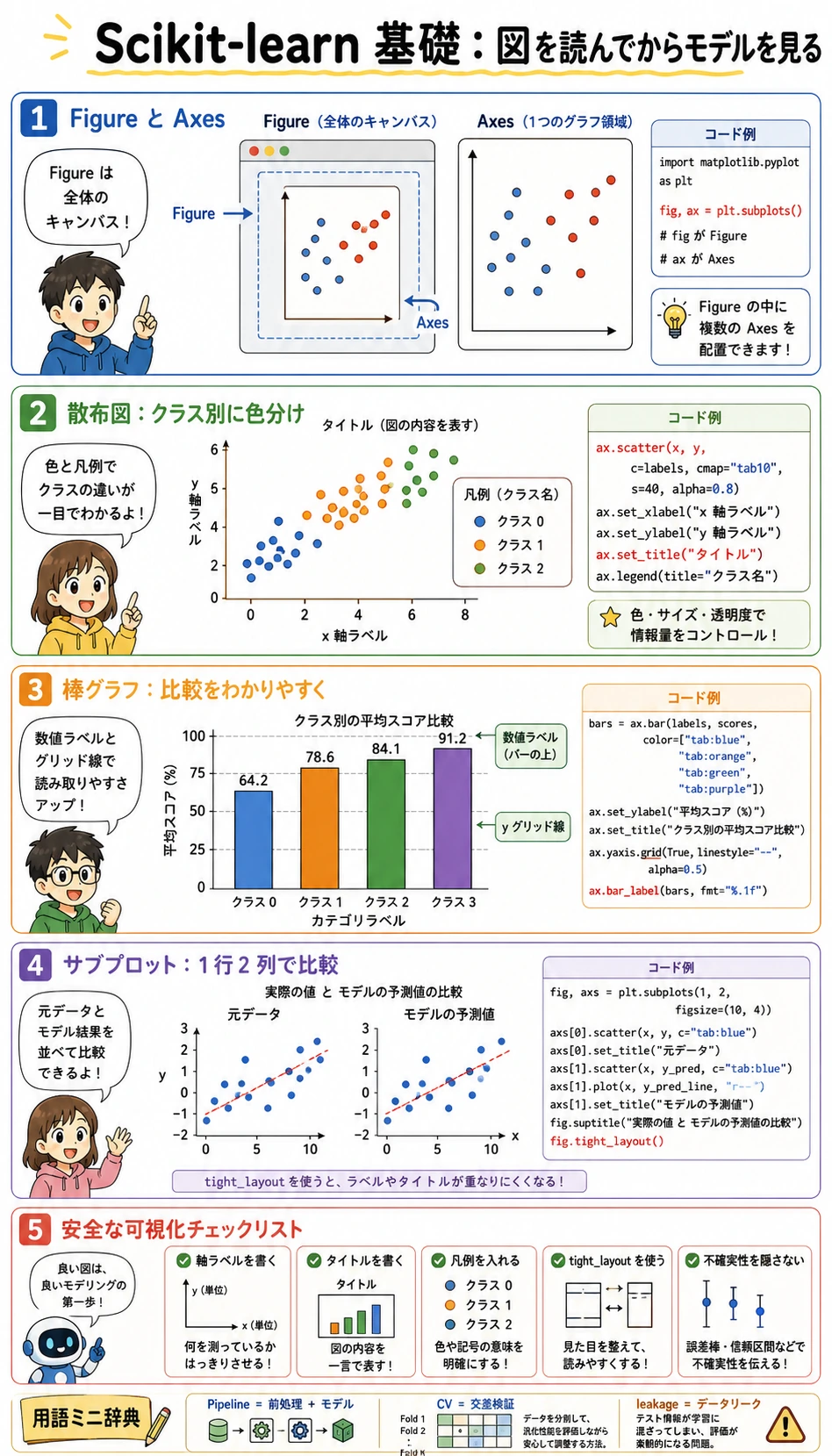
Matplotlib では、初心者が混乱しやすい言葉が2つあります。

• Figure：全体のキャンバスです。
• Axes：キャンバス内の1つのグラフ領域です。

入門段階では、次の形をよく使います。

fig, ax = plt.subplots(figsize=(6, 4))
ax.scatter(x_values, y_values)
ax.set_xlabel("x-axis label")
ax.set_ylabel("y-axis label")
ax.set_title("Chart title")
ax.grid(True, alpha=0.3)
plt.tight_layout()
plt.show()

Wine データセットから2つの特徴量を描いてみます。

feature_x = 0  # alcohol
feature_y = 6  # flavanoids

fig, ax = plt.subplots(figsize=(7, 5))
scatter = ax.scatter(
    X[:, feature_x],
    X[:, feature_y],
    c=y,
    cmap="viridis",
    s=45,
    alpha=0.85,
)

ax.set_xlabel(wine.feature_names[feature_x])
ax.set_ylabel(wine.feature_names[feature_y])
ax.set_title("Wine data: two-feature view")
ax.grid(True, alpha=0.3)
ax.legend(
    handles=scatter.legend_elements()[0],
    labels=wine.target_names.tolist(),
    title="Class",
)

plt.tight_layout()
plt.show()

見るポイントは次の通りです。

• クラスは少し分かれて見えるか？
• 重なっている領域はあるか？
• 数値範囲が極端に大きい特徴量はあるか？

可視化の価値は、モデルスコアを見る前に、問題の難しさを肌感覚でつかめることです。

---

データ分割：テストセットを隠しておく

train_test_split は訓練セットとテストセットを作ります。

• 訓練セット：モデルが学習してよいデータです。
• テストセット：最後の評価にだけ使うデータです。
• stratify=y：訓練とテストでクラス比率を近く保ちます。
• random_state：同じ分割を再現できるようにします。

X_train, X_test, y_train, y_test = train_test_split(
    X,
    y,
    test_size=0.2,
    random_state=42,
    stratify=y,
)

print("X_train:", X_train.shape, "y_train:", y_train.shape)
print("X_test: ", X_test.shape, "y_test: ", y_test.shape)

期待される出力：

X_train: (142, 13) y_train: (142,)
X_test:  (36, 13) y_test:  (36,)

よくある初心者ミス

テストセットで fit してはいけません。テストセットは最後の試験です。前処理や調整がテストセットから学んでしまうと、スコアが実力以上によく見えます。

---

Pipeline を作る：前処理とモデルをまとめる

ロジスティック回帰、SVM、KNN などは特徴量のスケールに敏感です。Wine データセットは列ごとの単位がかなり違うため、モデルの前に StandardScaler を置きます。

model = make_pipeline(
    StandardScaler(),
    LogisticRegression(max_iter=1000, random_state=42),
)

model.fit(X_train, y_train)

train_score = model.score(X_train, y_train)
test_score = model.score(X_test, y_test)

print(f"Train accuracy: {train_score:.1%}")
print(f"Test accuracy:  {test_score:.1%}")

期待される出力：

Train accuracy: 100.0%
Test accuracy:  100.0%

Pipeline が大事なのは、正しい順番を保てるからです。

1. 訓練データでは、StandardScaler.fit_transform のあとにモデルの fit
2. テストデータでは、StandardScaler.transform のあとにモデルの predict

この違いがデータリークを防ぎます。

---

予測し、具体例を見る

スコアだけでなく、実際の予測例も少し確認しましょう。

y_pred = model.predict(X_test)
proba = model.predict_proba(X_test[:5])

for i in range(5):
    predicted_name = wine.target_names[y_pred[i]]
    true_name = wine.target_names[y_test[i]]
    confidence = proba[i].max()
    print(f"Sample {i}: predicted={predicted_name}, true={true_name}, confidence={confidence:.1%}")

出力例：

Sample 0: predicted=class_0, true=class_0, confidence=99.9%
Sample 1: predicted=class_1, true=class_1, confidence=99.9%
Sample 2: predicted=class_0, true=class_0, confidence=99.5%
Sample 3: predicted=class_1, true=class_1, confidence=99.7%
Sample 4: predicted=class_2, true=class_2, confidence=99.9%

predict は最終クラスを返します。predict_proba は各クラスの確率分布を返します。確率は、しきい値、手動確認、リスク順位付けなどで役立ちます。

---

混同行列とレポートで評価する

Accuracy だけでは、どのクラスを間違えたのかが見えません。混同行列は、実ラベルと予測ラベルを表にして見せます。

fig, ax = plt.subplots(figsize=(5, 5))
ConfusionMatrixDisplay.from_estimator(
    model,
    X_test,
    y_test,
    display_labels=wine.target_names,
    cmap="Blues",
    ax=ax,
    colorbar=False,
)
ax.set_title("Confusion matrix on test set")
plt.tight_layout()
plt.show()

print(classification_report(y_test, y_pred, target_names=wine.target_names))

読み方：

• 対角線は正しく予測できた数です。
• 対角線以外は間違いです。
• Precision は「A と予測したもののうち、本当に A だった割合」です。
• Recall は「本当に A だったもののうち、どれだけ見つけたか」です。
• F1 は precision と recall をまとめた指標です。

---

同じ流れで複数モデルを比べる

sklearn は API が統一されているため、モデル比較がしやすいです。

from sklearn.tree import DecisionTreeClassifier
from sklearn.neighbors import KNeighborsClassifier
from sklearn.svm import SVC

models = {
    "Logistic Regression": make_pipeline(
        StandardScaler(),
        LogisticRegression(max_iter=1000, random_state=42),
    ),
    "Decision Tree": DecisionTreeClassifier(max_depth=4, random_state=42),
    "KNN": make_pipeline(StandardScaler(), KNeighborsClassifier(n_neighbors=5)),
    "SVM": make_pipeline(StandardScaler(), SVC(kernel="rbf", C=1.0, gamma="scale")),
}

results = {}
for name, clf in models.items():
    clf.fit(X_train, y_train)
    results[name] = {
        "train": clf.score(X_train, y_train),
        "test": clf.score(X_test, y_test),
    }
    print(f"{name:20s} train={results[name]['train']:.1%} test={results[name]['test']:.1%}")

出力例：

Logistic Regression  train=100.0% test=100.0%
Decision Tree        train=99.3% test=94.4%
KNN                  train=97.9% test=97.2%
SVM                  train=100.0% test=100.0%

比較を棒グラフで描きます。

fig, ax = plt.subplots(figsize=(9, 5))
names = list(results.keys())
x = np.arange(len(names))
width = 0.35

train_scores = [results[name]["train"] for name in names]
test_scores = [results[name]["test"] for name in names]

bars_train = ax.bar(x - width / 2, train_scores, width, label="Train", color="steelblue")
bars_test = ax.bar(x + width / 2, test_scores, width, label="Test", color="coral")

ax.set_xticks(x)
ax.set_xticklabels(names, rotation=15, ha="right")
ax.set_ylabel("Accuracy")
ax.set_title("Model comparison on Wine dataset")
ax.set_ylim(0.8, 1.05)
ax.legend()
ax.grid(axis="y", alpha=0.3)
ax.bar_label(bars_train, fmt="%.2f", padding=3)
ax.bar_label(bars_test, fmt="%.2f", padding=3)

plt.tight_layout()
plt.show()

訓練スコアがテストスコアより大きく高い場合は、過学習を疑います。両方低い場合は、未学習、特徴量不足、またはモデルが合っていない可能性があります。

---

交差検証で安全に調整する

テストセットを直接使ってハイパーパラメータを調整してはいけません。訓練セット内で交差検証を使います。

candidates = [0.01, 0.1, 1.0, 10.0, 100.0]

for C in candidates:
    clf = make_pipeline(
        StandardScaler(),
        LogisticRegression(C=C, max_iter=1000, random_state=42),
    )
    scores = cross_val_score(clf, X_train, y_train, cv=5, scoring="accuracy")
    print(f"C={C:<6} CV accuracy={scores.mean():.1%} ± {scores.std():.1%}")

出力例：

C=0.01   CV accuracy=95.8% ± 3.1%
C=0.1    CV accuracy=98.6% ± 1.8%
C=1.0    CV accuracy=98.6% ± 1.8%
C=10.0   CV accuracy=97.9% ± 2.6%
C=100.0  CV accuracy=97.9% ± 2.6%

具体的な結果より大事なのは、次の習慣です。

1. 先にテストセットを切り出し、触らない。
2. 訓練セットで交差検証を使って調整する。
3. 一番よい設定を選ぶ。
4. 全訓練データで最終モデルを学習する。
5. 最後にテストセットで一度だけ評価する。

---

最終 Pipeline を保存して読み込む

import joblib

final_model = make_pipeline(
    StandardScaler(),
    LogisticRegression(C=1.0, max_iter=1000, random_state=42),
)
final_model.fit(X_train, y_train)

joblib.dump(final_model, "wine_classifier.joblib")
loaded_model = joblib.load("wine_classifier.joblib")

same_predictions = np.array_equal(
    final_model.predict(X_test),
    loaded_model.predict(X_test),
)

print("Loaded model test accuracy:", f"{loaded_model.score(X_test, y_test):.1%}")
print("Predictions are identical:", same_predictions)

期待される出力：

Loaded model test accuracy: 100.0%
Predictions are identical: True

セキュリティ注意

信頼できる joblib や pickle ファイルだけを読み込んでください。Python のシリアライズ済みオブジェクトは、読み込み時にコードを実行する可能性があります。

---

よくあるエラーと直し方

エラー / 症状	よくある原因	修正方法
NameError: name 'X_train' is not defined	分割セルを実行していない	データ読み込みと train_test_split のセルを先に実行する
ValueError: Found input variables with inconsistent numbers of samples	X と y の長さが合っていない	分割前に X.shape と y.shape を表示する
訓練スコアは高いがテストスコアが低い	過学習	モデルを単純にする、交差検証を使う、データを増やす、特徴量を見直す
Notebook のスコアは良いが実運用で悪い	データリークまたは前処理の不一致	モデル単体ではなく、完全な Pipeline を保存して使う
グラフのラベルが重なる	図が小さい、またはレイアウト未調整	figsize を大きくする、ラベルを回転する、plt.tight_layout() を使う

手を動かす課題

load_iris() で同じ流れを繰り返しましょう。

1. X.shape、y.shape、特徴量名、クラス名を表示する。
2. 2つの特徴量で散布図を描く。
3. train_test_split(..., stratify=y) で分割する。
4. Pipeline(StandardScaler(), LogisticRegression(...)) を学習する。
5. 訓練 accuracy とテスト accuracy を表示する。
6. 混同行列を描く。
7. 交差検証で C を調整する。
8. joblib で保存し、再読み込みする。

この節で持ち帰ってほしいこと

第5章の実践ループをひとことで言うなら、これです。

まずデータを見る。分割してから fit する。Pipeline で前処理とモデルをつなぐ。隠したデータで評価する。交差検証で改善する。最後に完全なワークフローを保存する。