4.4 実践:第 4 章フル数学ワークショップ
このページでは、第 4 章を手を動かして進める 1 本の練習ルートにします。ここで全ての公式を証明する必要はありません。小さなスクリプトを動かし、重要な数学の直感を見える形にします。ベクトルは類似度を比べ、確率は不確実性を表し、エントロピーと loss は「どれくらい意外か」を測り、勾配はパラメータが進む方向を教えます。
スクリプトは Python 標準ライブラリだけを使います。初回実行では NumPy も描画ライブラリも Notebook 設定も不要です。それでも CSV、SVG 図、README を出力するので、小さなエンジニアリング成果物として数学を見直せます。
各ステップでは、先に図を見て、次にコードを実行し、最後に出力ファイルを確認します。公式が抽象的に感じるときは、それが何を表すのか、どんな不確実性を測るのか、どんな更新を案内するのかを考えてください。
作るもの
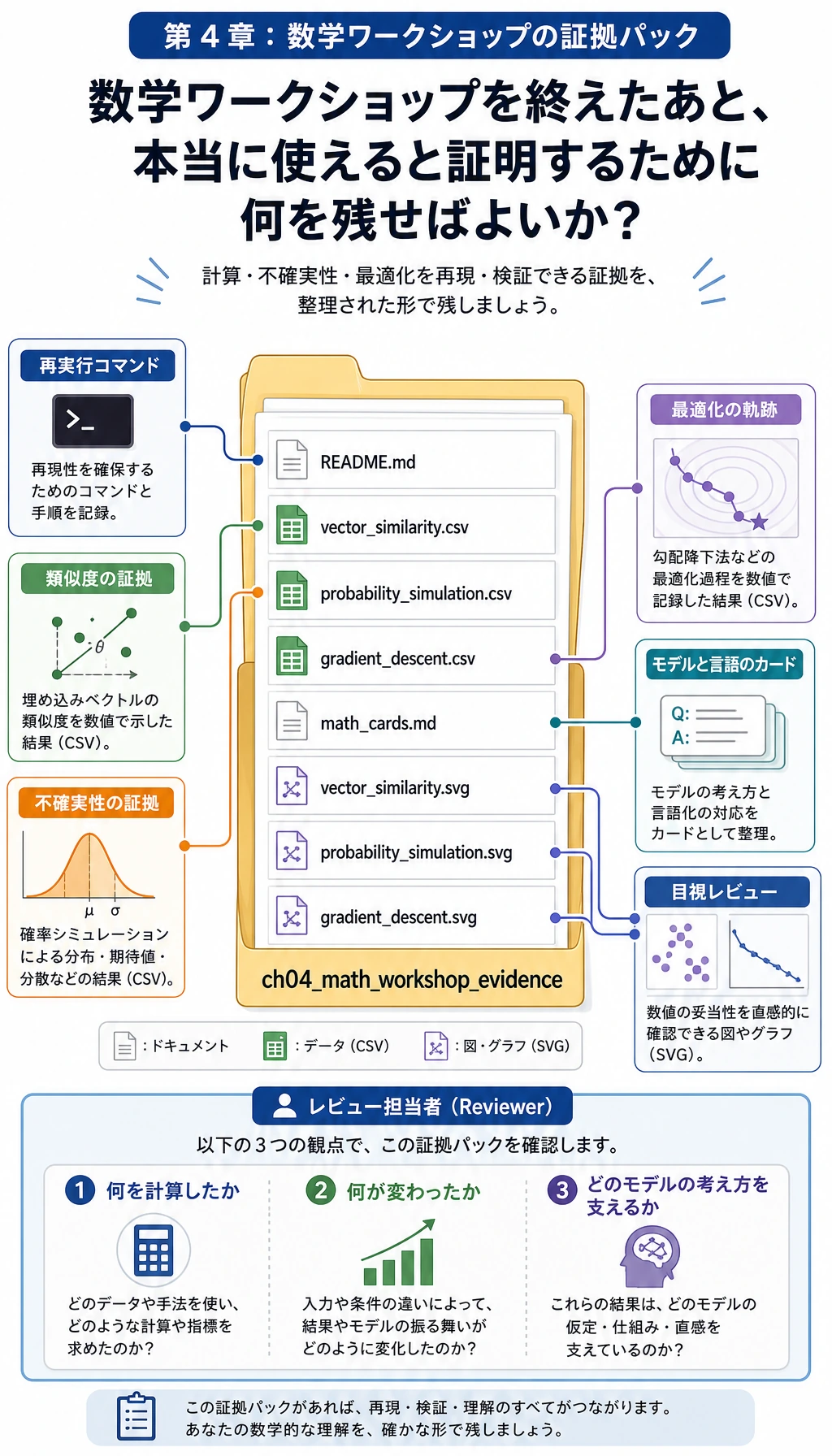
最後まで進めると、ch04_math_workshop_evidence というフォルダができます。
| ファイル | 何を示すか |
|---|---|
vector_similarity.csv | 小さなベクトルで dot product、norm、cosine similarity、distance を計算できる。 |
probability_simulation.csv | 繰り返しサンプリングをシミュレーションし、揺らぎを確認できる。 |
gradient_descent.csv | パラメータ更新を 1 ステップずつ追える。 |
math_cards.md | 公式を AI モデルの言葉に翻訳できる。 |
vector_similarity.svg | 公式だけでなく、ベクトル比較を図として確認できる。 |
probability_simulation.svg | 観測確率が期待確率の周辺で揺れる様子を見られる。 |
gradient_descent.svg | 最適化中に loss が下がる様子を見られる。 |
README.md | 再実行とレビューの方法を説明できる。 |
図解チェックポイント:全体ルート
コードを書く前に、次の図をワークショップの地図として見てください。
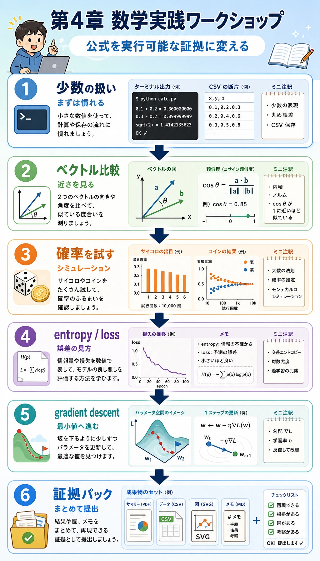
全体の流れは、小さな数値から始め、コードで動かし、最後に見える証拠を残すことです。
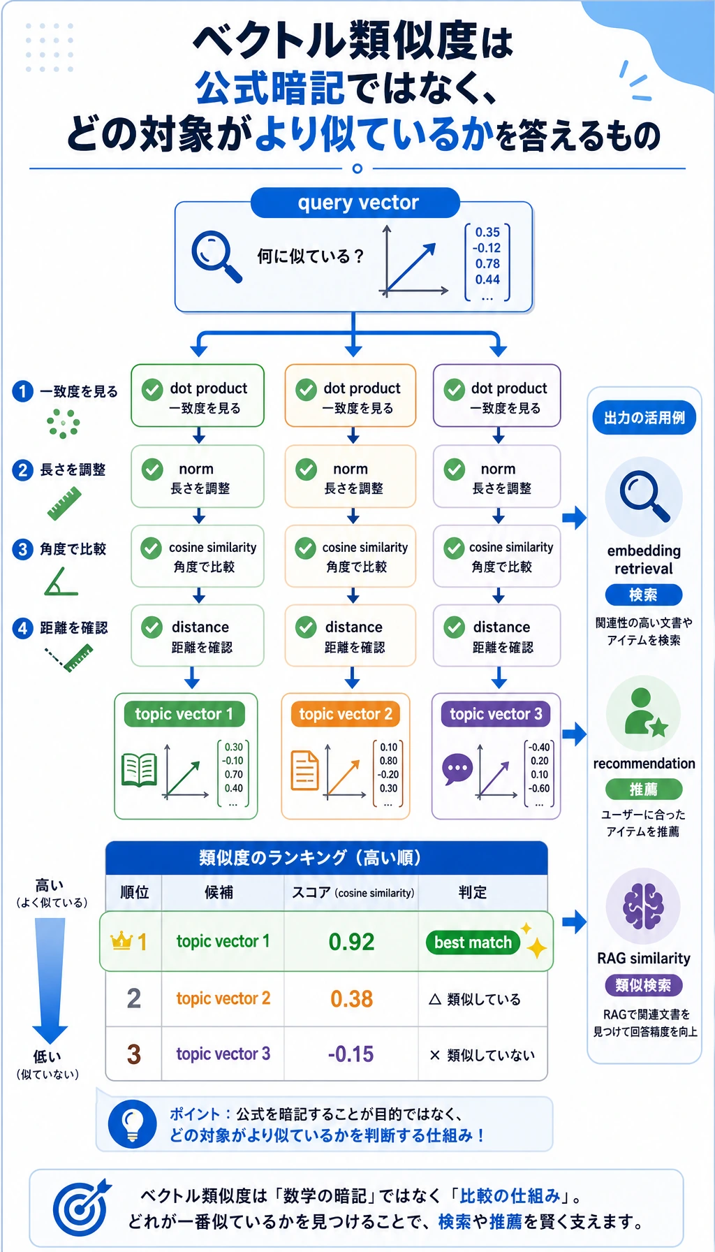
ベクトルのステップでは、クエリベクトルに最も近い向きを持つトピックを探します。
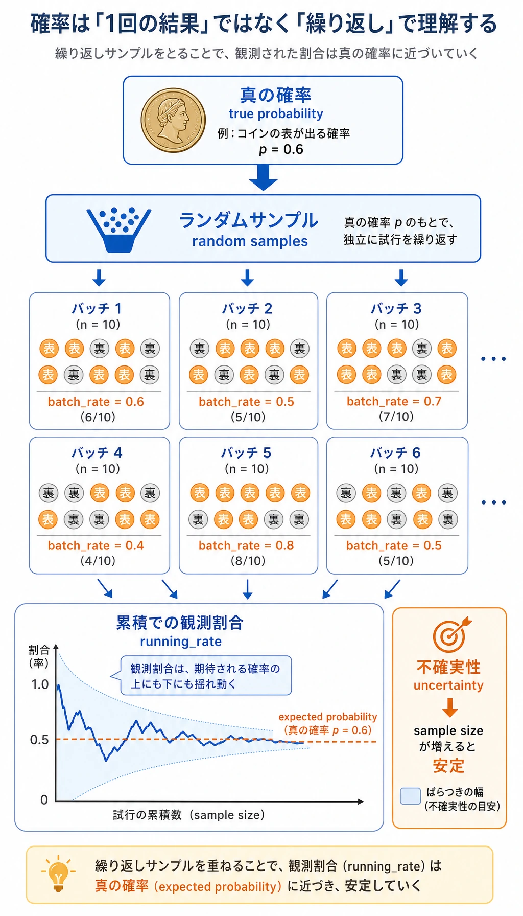
確率のステップでは、モデルスコアが魔法の正解ではなく、サンプル全体の不確実性を要約する方法だと分かります。
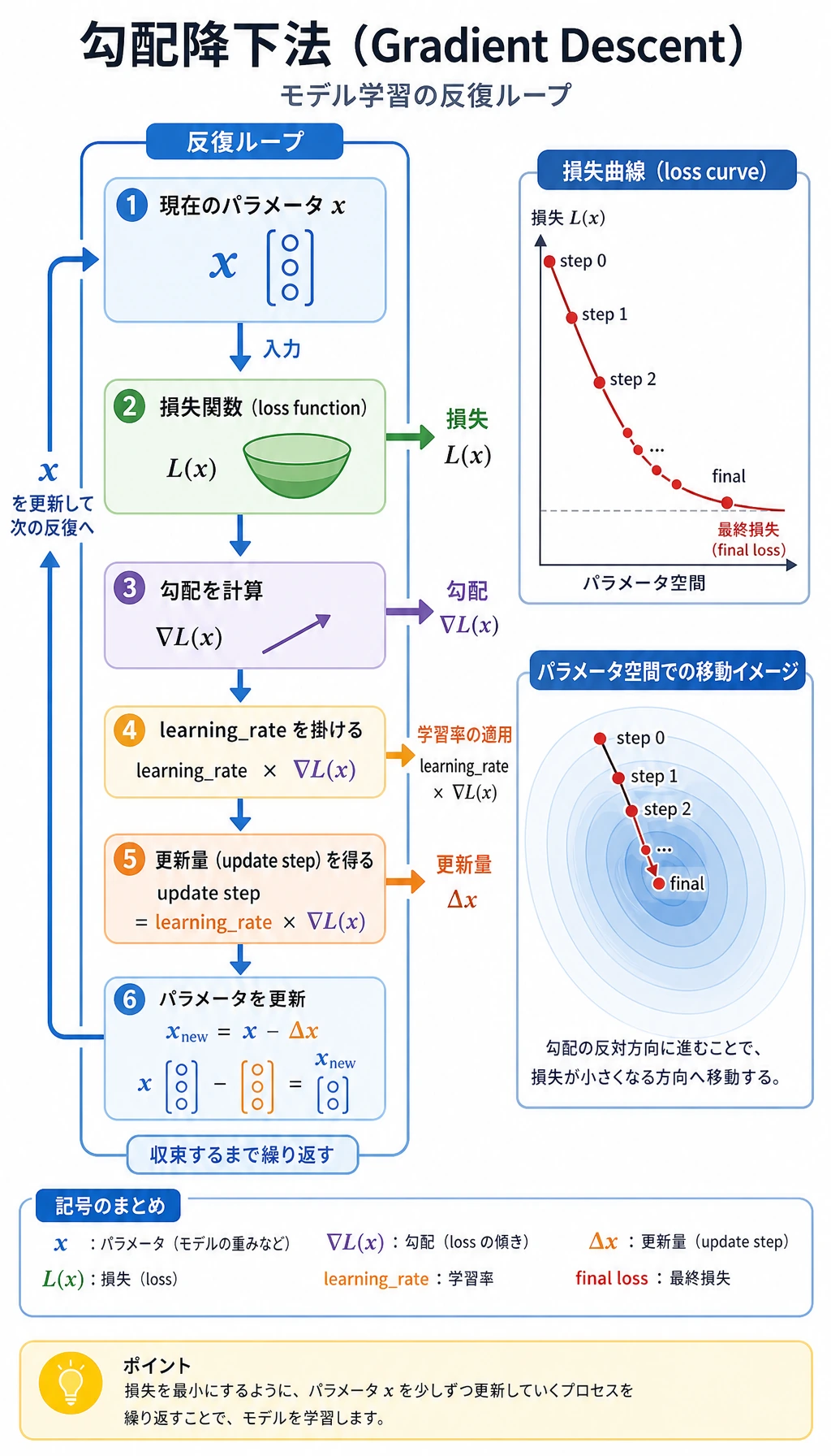
勾配降下のステップでは、loss を計算し、傾きを計算し、パラメータを更新し、繰り返すという訓練のリズムを見ます。
証拠フォルダは最終的な学習成果物です。記憶だけに頼らず、あとから数学を見直せます。
プロジェクトフォルダを作る
小さなローカルフォルダを作ります。
mkdir ch04_math_hands_on
cd ch04_math_hands_on
次に math_workshop.py というファイルを作成します。
ワークショップコードを貼り付けて実行する
次のコードを math_workshop.py に保存します。
import csv
import math
import random
from pathlib import Path


OUT_DIR = Path("ch04_math_workshop_evidence")

QUERY = ("ai_math_foundation", [1.0, 0.7, 0.2])
TOPICS = [
    ("vector_similarity", [1.0, 0.8, 0.1], "Embedding and retrieval need similarity."),
    ("probability", [0.2, 1.0, 0.7], "Classification confidence needs uncertainty."),
    ("gradient_descent", [0.8, 0.2, 1.0], "Training needs a direction of improvement."),
]


def dot(a, b):
    return sum(x * y for x, y in zip(a, b))


def norm(v):
    return math.sqrt(sum(x * x for x in v))


def cosine_similarity(a, b):
    return dot(a, b) / (norm(a) * norm(b))


def euclidean_distance(a, b):
    return math.sqrt(sum((x - y) ** 2 for x, y in zip(a, b)))


def run_vector_similarity():
    query_name, query = QUERY
    rows = []
    for topic, vector, note in TOPICS:
        rows.append(
            {
                "query": query_name,
                "topic": topic,
                "dot": round(dot(query, vector), 4),
                "query_norm": round(norm(query), 4),
                "topic_norm": round(norm(vector), 4),
                "cosine_similarity": round(cosine_similarity(query, vector), 4),
                "euclidean_distance": round(euclidean_distance(query, vector), 4),
                "model_language": note,
            }
        )
    return sorted(rows, key=lambda row: row["cosine_similarity"], reverse=True)


def run_probability_simulation(seed=42, batches=12, trials_per_batch=20, true_probability=0.65):
    random.seed(seed)
    rows = []
    running_successes = 0
    running_trials = 0
    for batch in range(1, batches + 1):
        successes = sum(1 for _ in range(trials_per_batch) if random.random() < true_probability)
        running_successes += successes
        running_trials += trials_per_batch
        rows.append(
            {
                "batch": batch,
                "batch_trials": trials_per_batch,
                "batch_successes": successes,
                "batch_rate": round(successes / trials_per_batch, 4),
                "running_rate": round(running_successes / running_trials, 4),
                "expected_probability": true_probability,
            }
        )
    return rows


def entropy(probabilities):
    return -sum(p * math.log2(p) for p in probabilities if p > 0)


def binary_cross_entropy(predicted_probability, actual_label):
    p = min(max(predicted_probability, 1e-9), 1 - 1e-9)
    return -(actual_label * math.log(p) + (1 - actual_label) * math.log(1 - p))


def run_information_examples():
    confident = [0.9, 0.1]
    uncertain = [0.5, 0.5]
    return {
        "entropy_confident_bits": round(entropy(confident), 4),
        "entropy_uncertain_bits": round(entropy(uncertain), 4),
        "loss_good_prediction": round(binary_cross_entropy(0.9, 1), 4),
        "loss_bad_prediction": round(binary_cross_entropy(0.2, 1), 4),
    }


def run_gradient_descent(start=3.5, learning_rate=0.2, steps=12):
    def loss(x):
        return (x - 1.4) ** 2 + 0.6

    def gradient(x):
        return 2 * (x - 1.4)

    x = start
    rows = []
    for step in range(steps + 1):
        current_loss = loss(x)
        current_gradient = gradient(x)
        rows.append(
            {
                "step": step,
                "x": round(x, 6),
                "loss": round(current_loss, 6),
                "gradient": round(current_gradient, 6),
                "learning_rate": learning_rate,
            }
        )
        x = x - learning_rate * current_gradient
    return rows


def write_csv(path, rows, fieldnames):
    with path.open("w", newline="", encoding="utf-8") as file:
        writer = csv.DictWriter(file, fieldnames=fieldnames)
        writer.writeheader()
        writer.writerows(rows)


def scale(value, old_min, old_max, new_min, new_max):
    if old_max == old_min:
        return (new_min + new_max) / 2
    ratio = (value - old_min) / (old_max - old_min)
    return new_min + ratio * (new_max - new_min)


def write_vector_svg(path, rows):
    width, height = 640, 420
    bars = []
    for index, row in enumerate(rows):
        bar_width = int(row["cosine_similarity"] * 360)
        y = 80 + index * 90
        bars.append(
            f'<text x="40" y="{y}" font-size="18">{row["topic"]}</text>'
            f'<rect x="240" y="{y - 22}" width="{bar_width}" height="28" fill="#4f8cff" />'
            f'<text x="{250 + bar_width}" y="{y}" font-size="16">{row["cosine_similarity"]}</text>'
        )
    svg = f'''<svg xmlns="http://www.w3.org/2000/svg" width="{width}" height="{height}" viewBox="0 0 {width} {height}">
<rect width="100%" height="100%" fill="#ffffff"/>
<text x="40" y="40" font-size="24" font-family="Arial">Vector similarity by cosine</text>
{''.join(bars)}
</svg>'''
    path.write_text(svg, encoding="utf-8")


def write_probability_svg(path, rows):
    width, height = 700, 420
    points = []
    for row in rows:
        x = scale(row["batch"], 1, len(rows), 70, 640)
        y = scale(row["running_rate"], 0.4, 0.9, 330, 80)
        points.append((x, y))
    polyline = " ".join(f"{x:.1f},{y:.1f}" for x, y in points)
    expected_y = scale(rows[0]["expected_probability"], 0.4, 0.9, 330, 80)
    circles = "".join(f'<circle cx="{x:.1f}" cy="{y:.1f}" r="5" fill="#f26d3d"/>' for x, y in points)
    svg = f'''<svg xmlns="http://www.w3.org/2000/svg" width="{width}" height="{height}" viewBox="0 0 {width} {height}">
<rect width="100%" height="100%" fill="#ffffff"/>
<text x="40" y="40" font-size="24" font-family="Arial">Running probability estimate</text>
<line x1="70" y1="{expected_y:.1f}" x2="640" y2="{expected_y:.1f}" stroke="#888" stroke-dasharray="8 6"/>
<text x="70" y="{expected_y - 10:.1f}" font-size="14">expected p=0.65</text>
<polyline points="{polyline}" fill="none" stroke="#f26d3d" stroke-width="3"/>
{circles}
</svg>'''
    path.write_text(svg, encoding="utf-8")


def write_gradient_svg(path, rows):
    width, height = 700, 420
    losses = [row["loss"] for row in rows]
    points = []
    for row in rows:
        x = scale(row["step"], 0, rows[-1]["step"], 70, 640)
        y = scale(row["loss"], min(losses), max(losses), 330, 80)
        points.append((x, y))
    polyline = " ".join(f"{x:.1f},{y:.1f}" for x, y in points)
    circles = "".join(f'<circle cx="{x:.1f}" cy="{y:.1f}" r="5" fill="#2f9e44"/>' for x, y in points)
    svg = f'''<svg xmlns="http://www.w3.org/2000/svg" width="{width}" height="{height}" viewBox="0 0 {width} {height}">
<rect width="100%" height="100%" fill="#ffffff"/>
<text x="40" y="40" font-size="24" font-family="Arial">Gradient descent lowers loss</text>
<polyline points="{polyline}" fill="none" stroke="#2f9e44" stroke-width="3"/>
{circles}
</svg>'''
    path.write_text(svg, encoding="utf-8")


def write_math_cards(path, info_examples):
    content = f"""# Math Cards

## Vector

Model language: a vector is a small numeric description of an object.
Workshop evidence: `vector_similarity.csv` shows which topic vector is closest to the query.

## Probability

Model language: probability is a controlled way to talk about uncertainty.
Workshop evidence: `probability_simulation.csv` shows observed rates moving around the expected rate.

## Entropy and Loss

Model language: entropy measures uncertainty; loss measures how painful a prediction mistake is.
Confident entropy: {info_examples['entropy_confident_bits']} bits.
Uncertain entropy: {info_examples['entropy_uncertain_bits']} bits.
Good prediction loss: {info_examples['loss_good_prediction']}.
Bad prediction loss: {info_examples['loss_bad_prediction']}.

## Gradient

Model language: a gradient tells a parameter which direction changes the loss fastest.
Workshop evidence: `gradient_descent.csv` shows x moving toward the low-loss point.
"""
    path.write_text(content, encoding="utf-8")


def write_readme(path, best_topic, final_gradient_row):
    content = f"""# Chapter 4 Math Workshop Evidence

Run command: `python math_workshop.py`

Best vector match: `{best_topic}`.
Final gradient descent point: x={final_gradient_row['x']}, loss={final_gradient_row['loss']}.

Review order:

1. Open `vector_similarity.csv`.
2. Open `probability_simulation.csv`.
3. Open `gradient_descent.csv`.
4. Read `math_cards.md`.
5. Inspect the SVG files.
"""
    path.write_text(content, encoding="utf-8")


def main():
    OUT_DIR.mkdir(exist_ok=True)

    vector_rows = run_vector_similarity()
    probability_rows = run_probability_simulation()
    info_examples = run_information_examples()
    gradient_rows = run_gradient_descent()

    write_csv(
        OUT_DIR / "vector_similarity.csv",
        vector_rows,
        ["query", "topic", "dot", "query_norm", "topic_norm", "cosine_similarity", "euclidean_distance", "model_language"],
    )
    write_csv(
        OUT_DIR / "probability_simulation.csv",
        probability_rows,
        ["batch", "batch_trials", "batch_successes", "batch_rate", "running_rate", "expected_probability"],
    )
    write_csv(
        OUT_DIR / "gradient_descent.csv",
        gradient_rows,
        ["step", "x", "loss", "gradient", "learning_rate"],
    )

    write_vector_svg(OUT_DIR / "vector_similarity.svg", vector_rows)
    write_probability_svg(OUT_DIR / "probability_simulation.svg", probability_rows)
    write_gradient_svg(OUT_DIR / "gradient_descent.svg", gradient_rows)
    write_math_cards(OUT_DIR / "math_cards.md", info_examples)
    write_readme(OUT_DIR / "README.md", vector_rows[0]["topic"], gradient_rows[-1])

    print("STEP 1: Vector similarity")
    print(f"best_match={vector_rows[0]['topic']} cosine={vector_rows[0]['cosine_similarity']}")

    print("\nSTEP 2: Probability simulation")
    print(f"final_running_rate={probability_rows[-1]['running_rate']} expected={probability_rows[-1]['expected_probability']}")

    print("\nSTEP 3: Entropy and loss")
    print(f"confident_entropy={info_examples['entropy_confident_bits']} uncertain_entropy={info_examples['entropy_uncertain_bits']}")
    print(f"good_loss={info_examples['loss_good_prediction']} bad_loss={info_examples['loss_bad_prediction']}")

    print("\nSTEP 4: Gradient descent")
    print(f"start_loss={gradient_rows[0]['loss']} final_x={gradient_rows[-1]['x']} final_loss={gradient_rows[-1]['loss']}")

    print("\nSTEP 5: Evidence files")
    for name in [
        "README.md",
        "vector_similarity.csv",
        "probability_simulation.csv",
        "gradient_descent.csv",
        "math_cards.md",
        "vector_similarity.svg",
        "probability_simulation.svg",
        "gradient_descent.svg",
    ]:
        print((OUT_DIR / name).as_posix())


if __name__ == "__main__":
    main()
実行します。
python math_workshop.py
環境で python3 を使う場合は、次を実行してください。
python3 math_workshop.py
期待される出力
次のような出力になれば大丈夫です。
STEP 1: Vector similarity
best_match=vector_similarity cosine=0.9944

STEP 2: Probability simulation
final_running_rate=0.6833 expected=0.65

STEP 3: Entropy and loss
confident_entropy=0.469 uncertain_entropy=1.0
good_loss=0.1054 bad_loss=1.6094

STEP 4: Gradient descent
start_loss=5.01 final_x=1.404571 final_loss=0.600021

STEP 5: Evidence files
ch04_math_workshop_evidence/README.md
ch04_math_workshop_evidence/vector_similarity.csv
ch04_math_workshop_evidence/probability_simulation.csv
ch04_math_workshop_evidence/gradient_descent.csv
ch04_math_workshop_evidence/math_cards.md
ch04_math_workshop_evidence/vector_similarity.svg
ch04_math_workshop_evidence/probability_simulation.svg
ch04_math_workshop_evidence/gradient_descent.svg
seed、学習率、ステップ数を変えた場合は、数値が少し変わっても問題ありません。
ファイルの読み方
まず vector_similarity.csv を開きます。最高スコアだけでなく、dot、cosine_similarity、euclidean_distance を比べてください。大事なのは、指標と質問を結びつけることです。同じ方向を見たいのか、同じ大きさを見たいのか、その両方を見たいのかを考えます。
次に probability_simulation.csv を開きます。batch_rate と running_rate を見てください。1 つの batch は大きく揺れますが、累積の比率はだんだん安定します。だからモデル評価では、サンプル数、評価セット、信頼度が重要になります。
最後に gradient_descent.csv を開きます。x、loss、gradient を順に追います。最初は勾配が大きく、x が低 loss の点に近づくほど小さくなります。これはモデル訓練の小さな数値版です。
各概念をモデルの言葉に翻訳する
| 概念 | 公式では | モデルの言葉では | ワークショップファイル |
|---|---|---|---|
| Vector | 数字のリスト | 対象をコンパクトに表す数値記述 | vector_similarity.csv |
| Dot product | 対応する成分を掛けて足す | 2 つの方向がどれくらい一致するか | vector_similarity.csv |
| Cosine similarity | dot product を長さで割る | 長さの影響を除いた類似度 | vector_similarity.csv |
| Probability | 0 から 1 の数 | 事象の起こりやすさ、または不確実性 | probability_simulation.csv |
| Entropy | 期待される驚き | 分布がどれくらい不確実か | math_cards.md |
| Cross-entropy loss | 誤った自信へのペナルティ | 予測ミスがどれくらい痛いか | math_cards.md |
| Gradient | 最も速く変化する方向 | パラメータが動くべき方向 | gradient_descent.csv |
初心者向けトラブルシューティング
| 症状 | ありそうな原因 | 対処 |
|---|---|---|
python: command not found | 環境では python3 を使う | python3 math_workshop.py を実行する |
| SVG がテキストとして開く | エディタが SVG の XML を開いている | ブラウザで開く |
| 確率の出力が少し違う | seed や試行回数を変えた | 文書どおりにするなら seed=42 を保つ |
| 勾配降下が大きく跳ねる | 学習率が大きすぎる | learning_rate=0.05 を試す |
| 勾配降下が遅すぎる | 学習率が小さすぎる | 安定版を見てから learning_rate=0.3 を試す |
| 数値の意味が分からない | モデル上の質問から切り離して読んでいる | これは類似度、不確実性、更新方向のどれかを先に考える |
ガイド付き練習
QUERYを[0.1, 1.0, 0.7]に変えます。どのトピックが最も近くなりますか。なぜですか。true_probabilityを0.65から0.5に変えます。累積比率はどう変わりますか。learning_rateを0.2から0.05に変えます。loss は下がり続けますか。速くなりますか、遅くなりますか。math_cards.mdに、行列積を自分の言葉で説明する節を追加します。- 各ファイルについて、後続章のどこにつながるかを 1 文で書きます。機械学習、深層学習、RAG、LLM のどれかに結びつけてください。
完了チェックリスト
- このワークショップをローカルで実行できる。
- ベクトル類似度が検索や推薦を支えられる理由を説明できる。
- 確率は 1 回の幸運な結果ではなく、繰り返しサンプルで見る必要がある理由を説明できる。
- 不確実な分布ほどエントロピーが大きい理由を説明できる。
- 勾配降下がパラメータを小さく更新する理由を説明できる。
- 証拠フォルダを保存し、各ファイルが何を示すか説明できる。
6 つすべてを確認できれば、第 4 章はただの公式の章ではなく、動かせるモデル直感ツールキットになります。